The purpose of this post is to learn about the Probably Approximately Correct Learning model introduced by Valiant in “A Theory of the Learnable.” This model is relevant because is the first formal framework to study the process of learning from a computational viewpoint. Computability theory and complexity theory became possible once we had a rigorous model of the phenomenon of mechanical calculations (Turing Machines) that could be used to explain the phenomenon and was valuable to study for its own sake. In this line, the phenomenon of learning is also very relevant and needs a model that is valuable in their own sake and also explain the process of learning and the limits of them. Valiant defines that a program to perform a task has been acquired by learning if it has been acquired by any means different to explicit programming.

Leslie Valiant

A learning game

In this section we are going to follow section 1.1 of Kearns book. Let us consider the following 1-player game of learning an axis aligned rectangle, that is, given an unknown axis aligned rectangle (\(\mathcal{R}\), called the target) in the euclidean plane the player receives from time to time a point of the plane \(p\), sampled from fixed and unknown distribution \(\mathcal{D}\), and a label that indicates if \(p\in \mathcal{R}\). The goal of the player is to select, using as little examples and computation as possible, a hypothesis rectangle \(\mathcal{R'}\) that approximates well the target rectangle \(\mathcal{R}\), we use as measure of error the probability of a point sampled from \(\mathcal{D}\) falling on \(\mathcal{R}\triangle \mathcal{R'}\).

A concrete situation that motives this game is that of learning the concept of "men of medium build". We will say that a man is of medium build if his height and weight both lie in some prescribed range, for example if his height is between 170 and 180 cm and his weight between 70 to 90 kg. The build of each man can be represented as a point in the plane with height and weight as coordinates and the concept of being of medium build is represented as a rectangle aligned with the axes. So to learn this concept, for a training period the learned is given examples of men and their dimensions and is told if them are of medium build or not. The learner needs to construct a hypothesis of the concept of men of medium build. After that the learner goes outside and walks around his city and sees every men with same probability, but even in that case, the points that represent their builds may not follow a uniform distribution, but a fixed distribution \(\mathcal{D}\). Evaluating the success of the learner is done by evaluating his success on classifying men in futures encounters, given that their follow the same distribution \(\mathcal{D}\) from where we sampled the examples during the training phase.

For this game there is a simple strategy for the learner, the strategy consists on requesting a sufficient large sample of size \(m\) and choose as \(\mathcal{R'}\) the the smallest axis aligned rectangle which contains all of the positives examples and none of the negatives examples. We say that this rectangle is the "tightest-fit rectangle"

Theorem 1.

For any target rectangle \(\mathcal{R}\) and for any distribution \(\mathcal{D}\), and for every values \(\epsilon > 0, \delta\leq \frac{1}{2}\) exists a value \(m\) of the sample size for which with probability \(1-\delta\) the tightest-fit rectangle has error at most \(\epsilon\)

Proof

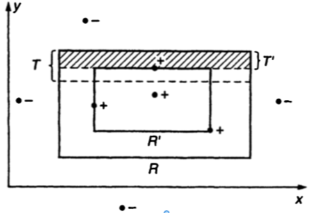
Remember that the error of \(\mathcal{R'}\) is defined as \(\mathbb{P}_{x \sim \mathcal{D}}(x\in \mathcal{R}\triangle \mathcal{R'} )\) and by definition of tightest-fit \(\mathcal{R'}\subseteq \mathcal{R}\) so the error is equal to \(\mathbb{P}_{x \sim \mathcal{D}}(x\in \mathcal{R}\setminus \mathcal{R'} )\). We can express the difference \(\mathcal{R}\setminus \mathcal{R'}\) as the union of 4 rectangular strips, for example the topmost of these strips, which is denoted T’ in the fig 1 is the region above the upper boundary of \(\mathcal{R'}\) extended to the left and right, but below the upper boundary of \(\mathcal{R}\). There is some overlap between these 4 rectangular strips at the corners. We will show that the weight of each strip, that is the probability with respect of \(\mathcal{D}\) of falling in each strip, is at most \(\frac{\epsilon}{4}\) (is clear that this bound is not tight). Without loss of generality we will analyze the top strip \(T'\)

Figure 1

Define T as the rectangular strip along the inside top of \(\mathcal{R}\) which encloses exactly weight \(\frac{\epsilon}{4}\) under \(\mathcal{D}\) (We take the upper side of \(\mathcal{R}\) and drag a rectangle going down, under assumptions of continuity of measures we can always find a rectangle with the exact area that we want). We note that the weight of \(T'\) exceds \(\frac{\epsilon}{4}\) iff \(T\subseteq T'\) (which is does not happen in the figure), furthermore \(\frac{\epsilon}{4}\) iff \(T\subseteq T'\) iff no point in \(T\) appears in the sample, (in the other case the point is on \(\mathcal{R'}\) by definition of tightest fit).

By the definition of \(T\) the probability that a single draw from \(\mathcal{D}\) misses the region \(T\) is exactly \(1-\frac{\epsilon}{4}\), as the samples are independent and identically distributed, the probability that \(m\) draws from \(\mathcal{D}\) all miss the region is exactly \((1-\frac{\epsilon}{4})^{m}\). This analysis also applies to the other 3 strips, so the probability of falling in any of the strips is less than \(4(1-\frac{\epsilon}{4})^{m}\). To prove our claim only last to show that we can choose an \(m\) that satisfy \(4(1-\frac{\epsilon}{4})^{m}\leq \delta\). Now we remember the famous inequality that \((1-x)\leq e^{-x}\) and we deduce that \(4(1-\frac{\epsilon}{4})^{m}\leq 4 e^{\frac{-\epsilon m}{4}}\), and using logartims we conclude that \(m\geq \frac{4}{\epsilon} ln(\frac{4}{\delta})\) satisfy what we are looking.

The previous result shows that our strategy only needs a sample of size \(\frac{4}{\epsilon} ln(\frac{4}{\delta})\) to find a hypothesis rectangle that with probability of \(1-\delta\) will have a error of classification with probability at most \(\epsilon\). Also, the only assumptions about the distribution of the sample, is that their are i.i.d, we do not need a condition onto the distribution itself. On the other hand, if we want to increase accuracy by reducing \(\epsilon\) or to increase confidence by reducing \(\delta\), the number of examples that we need grows slowly, linearly on \(\frac{1}{\epsilon}\) and linearly on \(\frac{1}{\delta}\). Finally, the amount of computation that we need to build \(\mathcal{R'}\) given the examples is low.

The general PAC model

Now we will introduce the general PAC model, and for this we need some definitions.

We will call a set X the Instance Space, we think of it as the codifications of objects in the learner world.

A concept over X is a subset \(c\subset X\) of the instance space. Equivalently we can define a concept as a boolean function \(c: X\rightarrow\{0,1\}\) such that \(c(x)=1\) means that \(x\) is a positive example, and \(c(x)=0\) that is a negative example.

A concept class \(\mathcal{C}\) over X is a collection of concepts over X.

In our model, a learning algorithm will have access to positive and negative examples of an unknown Target Concept \(c \in \mathcal{C}\) where \(\mathcal{C}\) is a \(\textbf{known}\) concept class. The examples follow a fixed distribution \(\mathcal{D}\) We will define the error of the algorithm as follows.

Given a concept \(h\in X\) and a target concept \(c\), and a distribution \(\mathcal{D}\) the \(\textbf{error}\) between \(h\) and \(c\) is defined as \(error(h) = \mathbb{P}_{x\sim \mathcal{D}}(c(x)\neq h(x))\)

we will denote as \(EX(c,\mathcal{C})\) an oracle that runs in unit time and on each call returns a labeled example \((x, c(x))\) where \(x\) is drawn i.i.d from \(\mathcal{D}\)

Now we can finally define the PAC model, note that this definition is the original definition of the model but has been modified in the literature for issues of representation of concepts (see 1.22 of Kearns for details)

The PAC model

Let \(\mathcal{C}\) a concept class over X. We say that \(\mathcal{C}\) is PAC learnable if there exists an algorithm \(L\) with the following property: for every concept \(c\in \mathcal{C}\), for ev­ery distribution \(\mathcal{D}\) on X and for all \(0 \leq \epsilon, \delta \leq \frac{1}{2}\) if \(L\) is given access to \(EX(c,\mathcal{C})\) and inputs \(\epsilon\) and \(\delta\), then with probability \(1-\delta\), \(L\) outputs a hypothesis concept \(h\in \mathcal{C}\) with \(error(h)\leq \epsilon\) This probability is taken over the random examples drawn by calls to EX(c, D), and any internal randomization of L.

if L runs in time polynomial in \(\frac{1}{\epsilon}\) and \(\frac{1}{\delta}\) we say that \(\mathcal{C}\) is effi­ciently PAC learnable.

Given that definition, theorem 1 says that the concept class of axis-aligned rectangles over the euclidean plane is efficiently PAC learnable

Conjuntion of boolean literals is efficiently PAC learnable

Let consider the instance space \(X_{n}=\{0,1\}^{n}\), and each element of the space is interpreted as an assignment to the \(n\) boolean variables \(x_{1}\cdots x_{n}\). Let consider the concept class \(\mathcal{C}_{n}\) to be the class of all conjunctions of literals over \(x_{1}\cdots x_{n}\). We want to prove the following theorem.

Theorem 2.

The concept class of conjunctions of boolean literals is efficiently PAC learnable

Proof

We propose the following algorithm, start with the hypothesis \(h = x_{1}\land \neg x_{1} \land \cdots \land x_{n} \land \neg x_{n}\) note that initially \(h\) is unsatisfacible, the algorithm will ignore every negative example returned by \(EX(c,\mathcal{C})\). In case of a positive example \((a,1)\) the algorithm will update \(h\) as follows. For each \(i\), if \(a_{i}=0\), the algorithm will delete \(x_{i}\) from \(h\), and if \(a_{i}=0\), will delete \(\neg x_{i}\) from \(h\).That is, the algorithm will delete every literal that contradicts the positive data.

We need to prove that runs in time polynomial on \(\frac{1}{\epsilon}\) and \(\frac{1}{\delta}\)

First we note that the set of literals that appears in \(h\) always contains the set of literals on the target \(c\), because we start in \(h\) with all literals and remove from \(h\) only when they are set to in a positive example, so \(h\) only can fail on positive examples of \(c\). Consider a literal \(z\) that occurs in \(h\) but not in \(c\), then \(z\) causes \(h\) to err only in the positive examples of \(c\) in which \(z=0\). Note that this examples would have made that the algorithm deleted \(z\) from \(h\). Consider the probability of this examples, that is \(p(z) = \mathbb{P}_{a\sim \mathcal{D}}(c(a)=1 \land z\text{ is 0 in } a )\). Since every error of \(h\) is caused by at least one literal \(z\) of \(h\), we have that \(error(h)\leq \sum_{z\in h} p(z)\). We will say that a literal is bad if \(p(z)\geq \frac{\epsilon}{2n}\). Observe that as \(h\) has at most \(2n\) literals, if \(h\) contains no bad literals then \(error(h)\leq \sum_{z\in h} p(z)\leq 2n\frac{\epsilon}{2n}=\epsilon\).

Now we are going to upper bound the probability of that \(h\) contains a bad literal. The probability of deleting a literal is \(p(z)\), and for a fixed bad literal that is at least \(\frac{\epsilon}{2n}\), so the probability of not deleting a fixed bad literal in a call to the oracle is \(1-\frac{\epsilon}{2n}\), and after \(m\) calls is \((1-\frac{\epsilon}{2n})^{m}\). This is for a fixed bad literal, and exists at most \(2n\) posible literals, so the probability of that there is some bad literal on \(h\) after \(m\) calls is bounded above by \(2n(1-\frac{\epsilon}{2n})^{m}\), so we now need to find the value of \(m\) that satisfies \(2n(1-\frac{\epsilon}{2n})^{m}\leq \delta\), we use the famous inequality that \((1-x)\leq e^{-x}\) and find that suffices to pick \(m\) such that \(2ne^{\frac{-m\epsilon}{2n}}\leq \delta\), and we conclude that we need \(m\geq (\frac{2n}{\epsilon})(ln(2n)+ln(\frac{1}{\delta}))\).

The bound above says that with a number of examples greater than \((\frac{2n}{\epsilon})(ln(2n)+ln(\frac{1}{\delta}))\) with probability \(1-\delta\) the error of h will be less than \(\epsilon\). The algorithm takes linear time to process each example, so the running time is bounded by \(mn\), and that is polynomial in \(\frac{1}{\epsilon}\) and \(\frac{1}{\delta}\). That concludes the proof.

References

Leslie G. Valiant: A Theory of the Learnable. Commun. ACM 27(11): 1134-1142 (1984)

Michael J. Kearns, Umesh V. Vazirani: An Introduction to Computational Learning Theory. MIT Press 1994, ISBN 978-0-262-11193-5, pp. I-XII, 1-207